Data transformation is data preprocessing technique used to reorganize or restructure the raw data in such a way that the data mining retrieves strategic information efficiently and easily. Data transformation include data cleaning and data reduction processes such as smoothing, clustering, binning, regression, histogram etc.
In this section, we will study different strategies used to perform data transformation. We will try to understand each data transformation process or strategy with the help of an example.
Content: Data Transformation in Data Mining
What is Data Transformation?
Data transformation is a technique used to convert the raw data into a suitable format that eases data mining in retrieving the strategic information efficiently and fastly. Raw data is difficult to trace or understand that’s why it needs to be preprocessed before retrieving any information from it. Data transformation includes data cleaning techniques as well as a data reduction technique to convert the data into the appropriate form.
Data transformation is one of the essential data preprocessing technique that must be performed on the data before data mining in order to provide patterns that are easier to understand. Knowing data transformation let’s move toward the strategies involved in data transformation.
Data Transformation Strategies
Let us study strategies used for data transformation in brief some of which we have already studied in data reduction and data cleaning.
1. Data Smoothing
We have studied this technique of data smoothing in our previous content ‘data cleaning’. Smoothing the data means removing noise from the considered data set. There we have seen how the noise is removed from the data using the techniques such as binning, regression, clustering.
- Binning: This method splits the sorted data into the number of bins and smoothens the data values in each bin considering the neighbourhood values around it.
- Regression: This method identifies the relation among two dependent attributes so that if we have one attribute it can be used to predict the other attribute.
- Clustering: This method groups, similar data values and form a cluster. The values that lie outside a cluster are termed as outliers.
2. Attribute Construction
In attribute construction method, the new attributes are constructed consulting the existing set of attributes in order to construct a new data set that eases data mining.
This can be understood with the help on an example, consider we have a data set referring to measurements of different plots i.e. we may have height and width of each plot. So here we can construct a new attribute ‘area’ from attributes ‘height’ and ‘weight’. This also helps in understanding the relations among the attributes in a data set.
3. Data Aggregation
Data aggregation transforms a large set of data to a smaller volume by implementing aggregation operation on the data set.
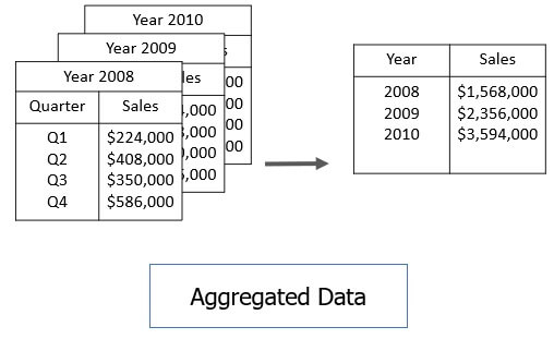
For example, we have a data set of sales reports of an enterprise that has quarterly sales of each year. We can aggregate the data in order to get the annual sales report of the enterprise.
4. Data Normalization
Normalizing the data refers to scaling the data values to a much smaller range like such as [-1, 1] or [0.0, 1.0]. There are different methods to normalize the data as discussed below.
For our further discussion consider that we have a numeric attribute A and we have n number of observed values for attribute A that are Ʋ1, Ʋ2, Ʋ3, ….Ʋn.
a. Min-max normalization
This method implements a linear transformation on the original data. Let us consider that we have minA and maxA as the minimum and maximum value observed for the attribute A and Ʋi is the value for attribute A that has to be normalized.
The min-max normalization would map Ʋi to the Ʋ’i, in a new smaller range [new_minA, new_maxA].
The formula for min-max normalization is:
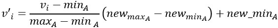 For example, we have $1200 and $9800 as the minimum and maximum value for the attribute ‘income’ and [0.0, 1.0] is the range in which we have to map a value $73,600.
The value $73,600 would be transformed using min-max normalization:
![]()
b. Z-score normalization
This method normalizes the value for attribute A using the mean and standard deviation. The formula for the same is:
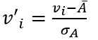 Here Ᾱ and σA are the mean and standard deviation for attribute A respectively.
Now, for example, we have a mean and standard deviation for attribute A as $54,000 and $16,000 respectively. And we have to normalize the value $73,600 using z-score normalization.
![]()
c. Decimal Scaling
This method normalizes the value of attribute A by moving the decimal point in the value. This movement of a decimal point depends on the maximum absolute value of A.
The formula for the decimal scaling is:
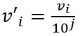 Here j is the smallest integer such that max(|v’i|)<1
For example, the observed values for attribute A lie in the range from -986 to 917 and the maximum absolute value for attribute A is 986. Here, to normalize each value of attribute A using decimal scaling, we have to divide each value of attribute A by 1000 i.e. j=3.
So, the value -986 would get normalized to -0.986 and 917 would get normalized to 0.917.
The normalization parameters such as mean, standard deviation, the maximum absolute value must be preserved in order to normalize the future data uniformly.
5. Data Discretization
Data discretization promotes the transformation of data by replacing the values of numeric data by the interval labels. Like the values for the attribute ‘age’ can be replaced by the interval labels such as (0-10, 11-20…) or (kid, youth, adult, senior).
Data discretization can be classified into two types supervised discretization where the class information is used and the other is unsupervised discretization which is based on which direction does the process proceed i.e. ‘top-down splitting strategy’ or ‘bottom-up merging strategy’.
Data discretization can be implemented on the data to be transformed using the methods discussed below:
a. Binning
We have already discussed the binning method in our data reduction content. Well, this method can also be used for data discretization and further for developing concept hierarchy.
The observed values for an attribute are distributed into a number of bins of equal-width or equal-frequency. Then the values in each bean are smoothened using bin mean or bin median.
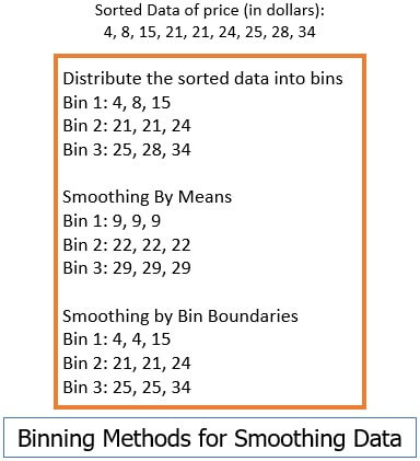 Using this method recursively you can generate concept hierarchy. Binning is unsupervised discretization as it does not use any class information.
b. Histogram Analysis
Histogram distribute the observed value of an attribute into disjoint subset which is also termed as buckets or bins.
Suppose have a data set for AllElectronics, where we have following observed values for the attribute ‘price’.
1, 1, 5, 5, 5, 5, 5, 8, 8, 10, 10, 10, 10, 12, 14, 14, 14, 15, 15, 15, 15, 15, 15, 18, 18, 18, 18, 18, 18, 18, 18, 20, 20, 20, 20, 20, 20, 20, 21, 21, 21, 21, 25, 25, 25, 25, 25, 28, 28, 30, 30, 30.
The histogram for the following could be shown as in the figure below.
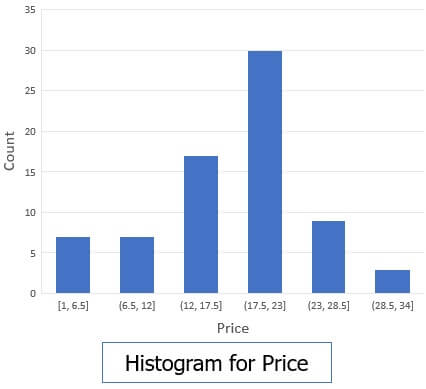 The histogram is also unsupervised discretization.
c. Cluster, Decision Tree and Correlation Analysis
We have studied cluster earlier as the attribute values are grouped into cluster depending on their closeness. Clustering can be implemented either using top-down or bottom-up strategy.
Generating a decision tree implements the top-down splitting strategy and is the supervised discretization. The class label information is used to identify the split points in the attribute values. We will discuss the decision tree in brief in our future contents.
Correlation analysis uses bottom-up merging strategy and for these, it analyzes the closest neighbourhood intervals and merges them to form a large interval. The merged intervals must be from same class label then only they can be merged.
6. Concept Hierarchy Generation for Nominal Data
The nominal data or the nominal attribute is one which has a finite number of unique values and there is no ordering between the values. Example for the nominal attribute is job-category, age-category, geographic-regions, items-category etc. The nominal attributes form the concept hierarchy by incorporating a group of attributes. Such as street, city, state, country all together can generate concept hierarchy.
Concept hierarchy converts the data into multiple levels. The concept hierarchy can be generated by introducing partial or total ordering between the attributes and this can be done at the schema level.
Concept hierarchy can also be generated by explicitly performing data grouping on a portion of the intermediate level of data. we can generate concept hierarchy by specifying a set of attributes but ignoring their ordering.
Key Takeaways
- Data transformation transforms the data into a suitable format that makes data mining efficient.
- Data transformation include method such as smoothing the data aggregation, attribute construction.
- The most effective way of transforming the data is normalizing and discretization and concept hierarchy.
- Data normalizing is scaling the data to a smaller range.
- Data discretization replaces the data values of a numeric attribute to interval labels.
- Concept hierarchy transforms the data into multiple levels.
So, this is all about data transformation and its strategies. Transforming data is important as it allow data mining to retrieve useful data efficiently.
Master Data Management Tools says
Very Informative Thankyou for sharing!